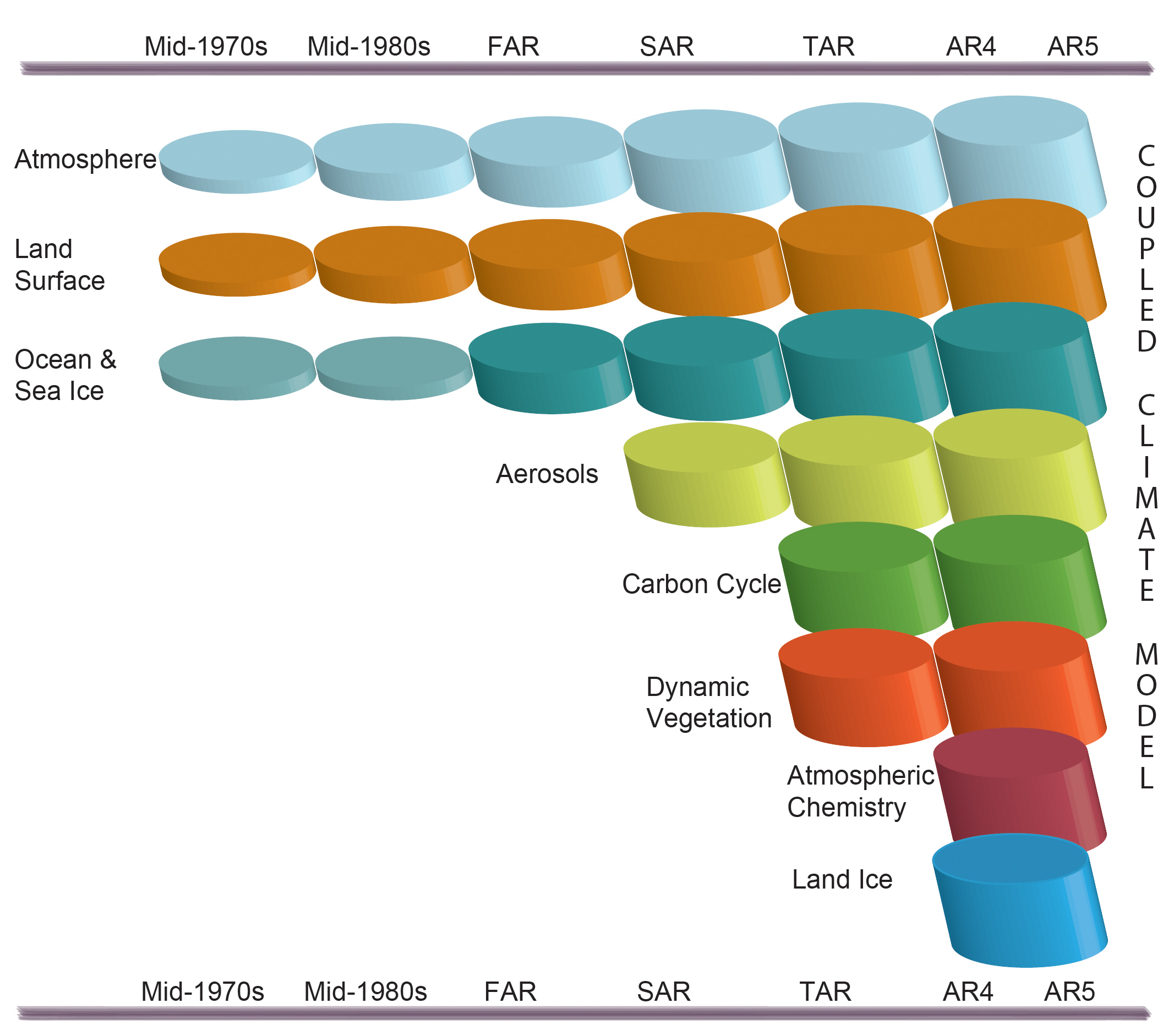
Figure 1.13 The development of climate models over the last 35 years showing how the different components were coupled into comprehensive climate models over time. In each aspect (e.g., the atmosphere, which comprises a wide range of atmospheric processes) the complexity and range of processes has increased over time (illustrated by growing cylinders). Note that during the same time the horizontal and vertical resolution has increased considerably e.g., for spectral models from T21L9 (roughly 500 km horizontal resolution and 9 vertical levels) in the 1970s to T95L95 (roughly 100 km horizontal resolution and 95 vertical levels) at present, and that now ensembles with at least three independent experiments can be considered as standard.
Several developments have especially pushed the capabilities in modelling forward over recent years (see Figure 1.13 and a more detailed discussion in Chapters 6, 7 and 9).

Figure 1.14 Horizontal resolutions considered in today's higher resolution models and in the very high resolution models now being tested: (a) Illustration of the European topography at a resolution of 87.5 x 87.5 km; (b) same as (a) but for a resolution of 30.0 x 30.0 km.
There has been a continuing increase in horizontal and vertical resolution. This is especially seen in how the ocean grids have been refined, and sophisticated grids are now used in the ocean and atmosphere models making optimal use of parallel computer architectures. More models with higher resolution are available for more regions. Figure 1.14a and 1.14b show the large effect on surface representation from a horizontal grid spacing of 87.5 km (higher resolution than most current global models and similar to that used in today’s highly resolved models) to a grid spacing of 30.0 km (similar to the current regional climate models).
Representations of Earth system processes are much more extensive and improved, particularly for the radiation and the aerosol cloud interactions and for the treatment of the cryosphere. The representation of the carbon cycle was added to a larger number of models and has been improved since AR4. A high-resolution stratosphere is now included in many models. Other ongoing process development in climate models includes the enhanced representation of nitrogen effects on the carbon cycle. As new processes or treatments are added to the models, they are also evaluated and tested relative to available observations (see Chapter 9 for more detailed discussion).
Ensemble techniques (multiple calculations to increase the statistical sample, to account for natural variability, and to account for uncertainty in model formulations) are being used more frequently, with larger samples and with different methods to generate the samples (different models, different physics, different initial conditions). Coordinated projects have been set up to generate and distribute large samples (ENSEMBLES, climateprediction.net, Program for Climate Model Diagnosis and Intercomparison).
The model comparisons with observations have pushed the analysis and development of the models. CMIP5, an important input to the AR5, has produced a multi-model data set that is designed to advance our understanding of climate variability and climate change. Building on previous CMIP efforts, such as the CMIP3 model analysis reported in AR4, CMIP5 includes ‘long-term’ simulations of 20th century climate and projections for the 21st century and beyond. See Chapters 9, 10, 11 and 12 for more details on the results derived from the CMIP5 archive.
Since AR4, the incorporation of ‘long-term’ paleoclimate simulations in the CMIP5 framework has allowed incorporation of information from paleoclimate data to inform projections. Within uncertainties associated with reconstructions of past climate variables from proxy records and forcings, paleoclimate information from the Mid Holocene, Last Glacial Maximum and Last Millennium have been used to test the ability of models to simulate realistically the magnitude and large scale patterns of past changes (Section 5.3, Box 5.1 and 9.4).
The capabilities of ESMs continue to be enhanced. For example, there are currently extensive efforts towards developing advanced treatments for the processes affecting ice sheet dynamics. Other enhancements are being aimed at land surface hydrology, and the effects of agriculture and urban environments.

Figure 1.15 Historical and projected total anthropogenic RF (W m–2) relative to preindustrial (about 1765) between 1950 and 2100. Previous IPCC assessments (SAR IS92a, TAR/ AR4 SRES A1B, A2 and B1) are compared with representative concentration pathway (RCP) scenarios (see Chapter 12 and Box 1.1 for their extensions until 2300 and Annex II for the values shown here). The total RF of the three families of scenarios, IS92, SRES and RCP, differ for example, for the year 2000, resulting from the knowledge about the emissions assumed having changed since the TAR and AR4.
As part of the process of getting model analyses for a range of alternative assumptions about how the future may unfold, scenarios for future emissions of important gases and aerosols have been generated for the IPCC assessments (e.g., see the SRES scenarios used in TAR and AR4). The emissions scenarios represent various development pathways based on well-defined assumptions. The scenarios are used to calculate future changes in climate, and are then archived in the Climate Model Intercomparison Project (e.g., CMIP3 for AR4; CMIP5 for AR5). For CMIP5, four new scenarios, referred to as Representative Concentration Pathways (RCPs) were developed (Section 12.3; Moss et al., 2010). See Box 1.1 for a more thorough discussion of the RCP scenarios. Because results from both CMIP3 and CMIP5 will be presented in the later chapters (e.g., Chapters 8, 9, 11 and 12), it is worthwhile considering the differences and similarities between the SRES and the RCP scenarios. Figure 1.15, acting as a prelude to the discussion in Box 1.1, shows that the RF for several of the SRES and RCP scenarios are similar over time and thus should provide results that can be used to compare climate modelling studies.
ES 1.1 1.2.1 1.2.2 1.2.3 1.3 1.3.1 1.3.2 1.3.3 1.3.4 1.3.4.1 1.3.4.2 1.3.4.3 1.4.1 1.4.2 1.4.3 1.4.4 1.5 1.5.1 1.5.2 1.6 Box 1 FAQ Refs