Here, some of the key concepts in climate science are briefly described; many of these were summarized more comprehensively in earlier IPCC assessments (Baede et al., 2001).[1] We focus only on a certain number of them to facilitate discussions in this assessment.
First, it is important to distinguish the meaning of weather from climate. Weather describes the conditions of the atmosphere at a certain place and time with reference to temperature, pressure, humidity, wind, and other key parameters (meteorological elements); the presence of clouds, precipitation; and the occurrence of special phenomena, such as thunderstorms, dust storms, tornados and others. Climate in a narrow sense is usually defined as the average weather, or more rigorously, as the statistical description in terms of the mean and variability of relevant quantities over a period of time ranging from months to thousands or millions of years. The relevant quantities are most often surface variables such as temperature, precipitation and wind. Classically the period for averaging these variables is 30 years, as defined by the World Meteorological Organization. Climate in a wider sense also includes not just the mean conditions, but also the associated statistics (frequency, magnitude, persistence, trends, etc.), often combining parameters to describe phenomena such as droughts. Climate change refers to a change in the state of the climate that can be identified (e.g., by using statistical tests) by changes in the mean and/or the variability of its properties, and that persists for an extended period, typically decades or longer.
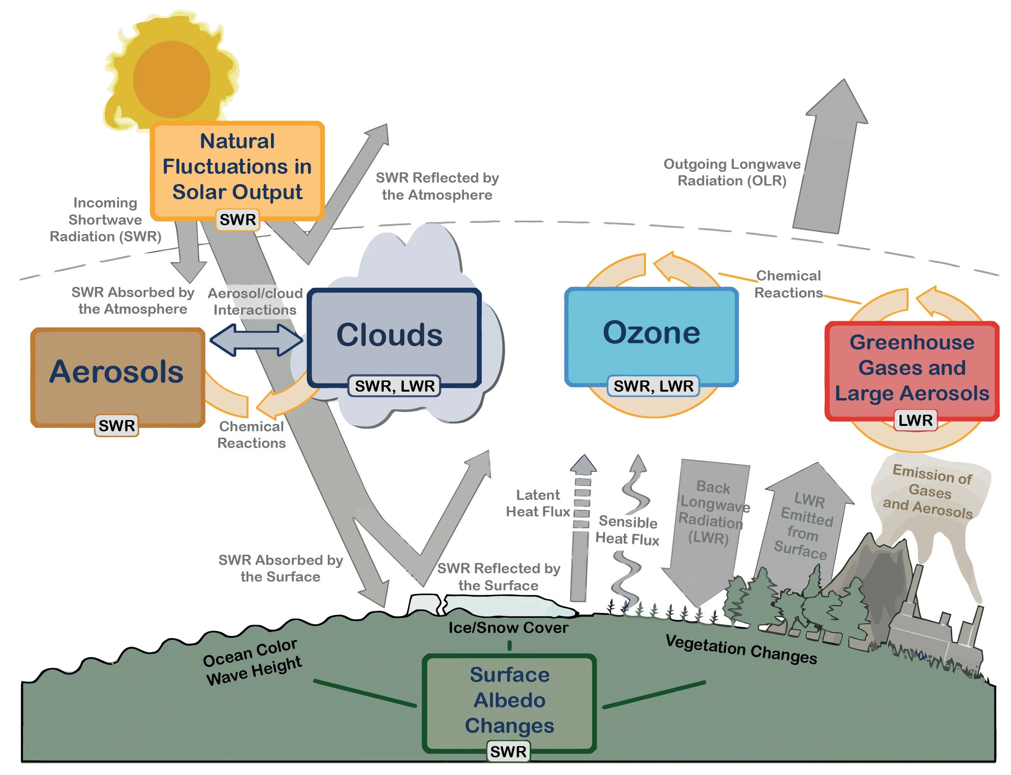
Figure 1.1. Main drivers of climate change. The radiative balance between incoming solar shortwave radiation (SWR) and outgoing longwave radiation (OLR) is influenced by global climate ‘drivers’. Natural fluctuations in solar output (solar cycles) can cause changes in the energy balance (through fluctuations in the amount of incoming SWR) (Section 2.3). Human activity changes the emissions of gases and aerosols, which are involved in atmospheric chemical reactions, resulting in modified O3 and aerosol amounts (Section 2.2). O3 and aerosol particles absorb, scatter and reflect SWR, changing the energy balance. Some aerosols act as cloud condensation nuclei modifying the properties of cloud droplets and possibly affecting precipitation (Section 7.4). Because cloud interactions with SWR and LWR are large, small changes in the properties of clouds have important implications for the radiative budget (Section 7.4). Anthropogenic changes in GHGs (e.g., CO2, CH4, N2O, O3, CFCs) and large aerosols (>2.5 μm in size) modify the amount of outgoing LWR by absorbing outgoing LWR and re-emitting less energy at a lower temperature (Section 2.2). Surface albedo is changed by changes in vegetation or land surface properties, snow or ice cover and ocean colour (Section 2.3). These changes are driven by natural seasonal and diurnal changes (e.g., snow cover), as well as human influence (e.g., changes in vegetation types) (Forster et al., 2007).
The Earth’s climate system is powered by solar radiation (Figure 1.1). Approximately half of the energy from the Sun is supplied in the visible part of the electromagnetic spectrum. As the Earth’s temperature has been relatively constant over many centuries, the incoming solar energy must be nearly in balance with outgoing radiation. Of the incoming solar shortwave radiation (SWR), about half is absorbed by the Earth’s surface. The fraction of SWR reflected back to space by gases and aerosols, clouds and by the Earth’s surface (albedo) is approximately 30%, and about 20% is absorbed in the atmosphere. Based on the temperature of the Earth’s surface the majority of the outgoing energy flux from the Earth is in the infrared part of the spectrum. The longwave radiation (LWR, also referred to as infrared radiation) emitted from the Earth’s surface is largely absorbed by certain atmospheric constituents—water vapour, carbon dioxide (CO2), methane (CH4), nitrous oxide (N2O) and other greenhouse gases (GHGs); see Annex III for Glossary—and clouds, which themselves emit LWR into all directions. The downward directed component of this LWR adds heat to the lower layers of the atmosphere and to the Earth’s surface (greenhouse effect). The dominant energy loss of the infrared radiation from the Earth is from higher layers of the troposphere. The Sun provides its energy to the Earth primarily in the tropics and the subtropics; this energy is then partially redistributed to middle and high latitudes by atmospheric and oceanic transport processes.
Changes in the global energy budget derive from either changes in the net incoming solar radiation or changes in the outgoing longwave radiation (OLR). Changes in the net incoming solar radiation derive from changes in the Sun’s output of energy or changes in the Earth’s albedo. Reliable measurements of total solar irradiance (TSI) can be made only from space, and the precise record extends back only to 1978. The generally accepted mean value of the TSI is about 1361 W/m2 (Kopp and Lean, 2011;[2] see Chapter 8 for a detailed discussion on the TSI); this is lower than the previous value of 1365 W/m2 used in the earlier assessments. Short-term variations of a few tenths of a percent are common during the approximately 11-year sunspot solar cycle (see Sections 5.2 and 8.4 for further details). Changes in the outgoing LWR can result from changes in the temperature of the Earth’s surface or atmosphere or changes in the emissivity (measure of emission efficiency) of LWR from either the atmosphere or the Earth’s surface. For the atmosphere, these changes in emissivity are due predominantly to changes in cloud cover and cloud properties, in GHGs and in aerosol concentrations. The radiative energy budget of the Earth is almost in balance (Figure 1.1), but ocean heat content and satellite measurements indicate a small positive imbalance (Murphy et al., 2009;[3] Trenberth et al., 2009;[4] Hansen et al., 2011[5]) that is consistent with the rapid changes in the atmospheric composition.
In addition, some aerosols increase atmospheric reflectivity, whereas others (e.g., particulate black carbon) are strong absorbers and also modify SWR (see Section 7.2 for a detailed assessment). Indirectly, aerosols also affect cloud albedo, because many aerosols serve as cloud condensation nuclei or ice nuclei. This means that changes in aerosol types and distribution can result in small but important changes in cloud albedo and lifetime (Section 7.4). Clouds play a critical role in climate because they not only can increase albedo, thereby cooling the planet, but also because of their warming effects through infrared radiative transfer. Whether the net radiative effect of a cloud is one of cooling or of warming depends on its physical properties (level of occurrence, vertical extent, water path and effective cloud particle size) as well as on the nature of the cloud condensation nuclei population (Section 7.3). Humans enhance the greenhouse effect directly by emitting GHGs such as CO2, CH4, N2O and chlorofluorocarbons (CFCs) (Figure 1.1). In addition, pollutants such as carbon monoxide (CO), volatile organic compounds (VOC), nitrogen oxides (NOx) and sulphur dioxide (SO2), which by themselves are negligible GHGs, have an indirect effect on the greenhouse effect by altering, through atmospheric chemical reactions, the abundance of important gases to the amount of outgoing LWR such as CH4 and ozone (O3), and/or by acting as precursors of secondary aerosols. Because anthropogenic emission sources simultaneously can emit some chemicals that affect climate and others that affect air pollution, including some that affect both, atmospheric chemistry and climate science are intrinsically linked.
In addition to changing the atmospheric concentrations of gases and aerosols, humans are affecting both the energy and water budget of the planet by changing the land surface, including redistributing the balance between latent and sensible heat fluxes (Sections 2.5, 7.2, 7.6 and 8.2). Land use changes, such as the conversion of forests to cultivated land, change the characteristics of vegetation, including its colour, seasonal growth and carbon content (Houghton, 2003;[6] Foley et al., 2005).[7] For example, clearing and burning a forest to prepare agricultural land reduces carbon storage in the vegetation, adds CO2 to the atmosphere, and changes the reflectivity of the land (surface albedo), rates of evapotranspiration and longwave emissions (Figure 1.1).
Changes in the atmosphere, land, ocean, biosphere and cryosphere— both natural and anthropogenic—can perturb the Earth’s radiation budget, producing a radiative forcing (RF) that affects climate. RF is a measure of the net change in the energy balance in response to an external perturbation. The drivers of changes in climate can include, for example, changes in the solar irradiance and changes in atmospheric trace gas and aerosol concentrations (Figure 1.1). The concept of RF cannot capture the interactions of anthropogenic aerosols and clouds, for example, and thus in addition to the RF as used in previous assessments, Sections 7.4 and 8.1 introduce a new concept, effective radiative forcing (ERF), that accounts for rapid response in the climate system. ERF is defined as the change in net downward flux at the top of the atmosphere after allowing for atmospheric temperatures, water vapour, clouds and land albedo to adjust, but with either sea surface temperatures (SSTs) and sea ice cover unchanged or with global mean surface temperature unchanged.
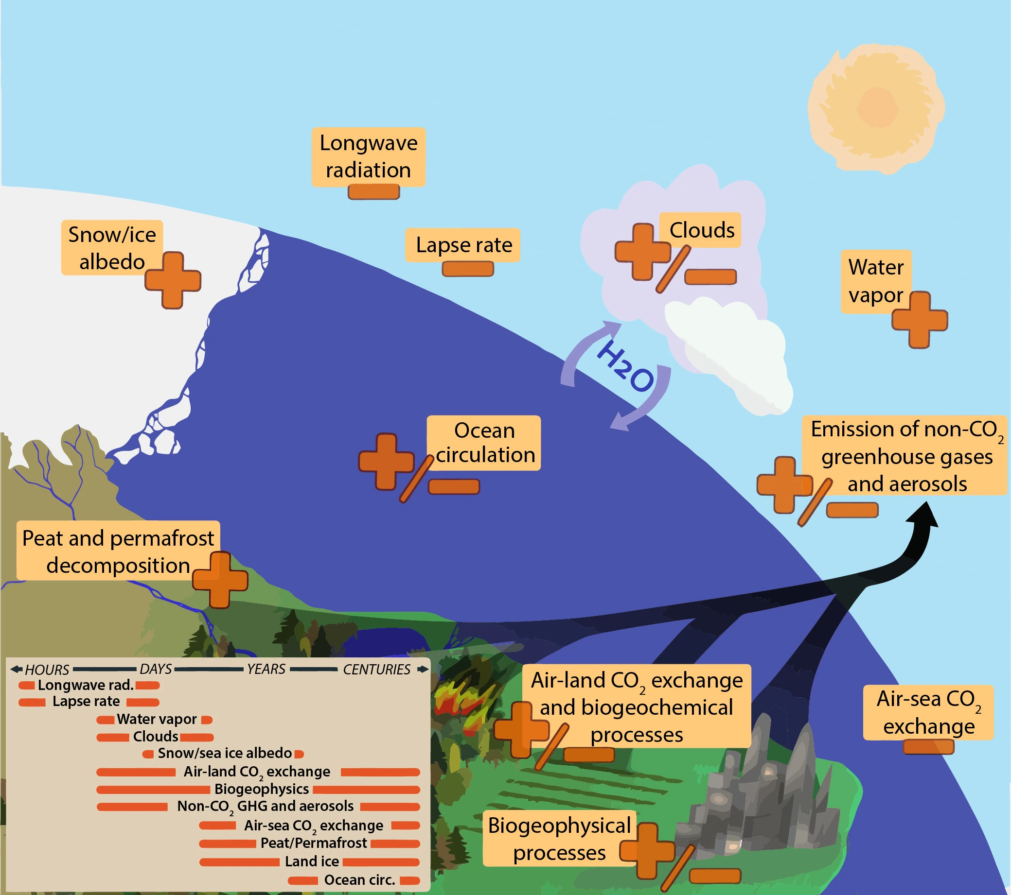
Figure 1.2 Climate feedbacks and timescales. The climate feedbacks related to increasing CO2 and rising temperature include negative feedbacks (–) such as LWR, lapse rate (see Glossary in Annex III), and air–sea carbon exchange and positive feedbacks (+) such as water vapour and snow/ice albedo feedbacks. Some feedbacks may be positive or negative (±): clouds, ocean circulation changes, air–land CO2 exchange, and emissions of non-GHGs and aerosols from natural systems. In the smaller box, the large difference in timescales for the various feedbacks is highlighted.
Once a forcing is applied, complex internal feedbacks determine the eventual response of the climate system, and will in general cause this response to differ from a simple linear one (IPCC, 2001, 2007). There are many feedback mechanisms in the climate system that can either amplify (‘positive feedback’) or diminish (‘negative feedback’) the effects of a change in climate forcing (Le Treut et al., 2007)[8] (see Figure 1.2 for a representation of some of the key feedbacks). An example of a positive feedback is the water vapour feedback whereby an increase in surface temperature enhances the amount of water vapour present in the atmosphere. Water vapour is a powerful GHG: increasing its atmospheric concentration enhances the greenhouse effect and leads to further surface warming. Another example is the ice albedo feedback, in which the albedo decreases as highly reflective ice and snow surfaces melt, exposing the darker and more absorbing surfaces below. The dominant negative feedback is the increased emission of energy through LWR as surface temperature increases (sometimes also referred to as blackbody radiation feedback). Some feedbacks operate quickly (hours), while others develop over decades to centuries; in order to understand the full impact of a feedback mechanism, its timescale needs to be considered. Melting of land ice sheets can take days to millennia.
A spectrum of models is used to project quantitatively the climate response to forcings. The simplest energy balance models use one box to represent the Earth system and solve the global energy balance to deduce globally averaged surface air temperature. At the other extreme, full complexity three-dimensional climate models include the explicit solution of energy, momentum and mass conservation equations at millions of points on the Earth in the atmosphere, land, ocean and cryosphere. More recently, capabilities for the explicit simulation of the biosphere, the carbon cycle and atmospheric chemistry have been added to the full complexity models, and these models are called Earth System Models (ESMs). Earth System Models of Intermediate Complexity include the same processes as ESMs, but at reduced resolution, and thus can be simulated for longer periods (see Annex III for Glossary and Section 9.1).
An equilibrium climate experiment is an experiment in which a climate model is allowed to adjust fully to a specified change in RF. Such experiments provide information on the difference between the initial and final states of the model simulated climate, but not on the time-dependent response. The equilibrium response in global mean surface air temperature to a doubling of atmospheric concentration of CO2 above pre-industrial levels (e.g., Arrhenius, 1896;[9] see Le Treut et al., 2007[8] for a comprehensive list) has often been used as the basis for the concept of equilibrium climate sensitivity (e.g., Hansen et al., 1981;[10] see Meehl et al., 2007[11] for a comprehensive list). For more realistic simulations of climate, changes in RF are applied gradually over time, for example, using historical reconstructions of the CO2, and these simulations are called transient simulations. The temperature response in these transient simulations is different than in an equilibrium simulation. The transient climate response is defined as the change in global surface temperature at the time of atmospheric CO2 doubling in a global coupled ocean–atmosphere climate model simulation where concentrations of CO2 were increased by 1% yr-1. The transient climate response is a measure of the strength and rapidity of the surface temperature response to GHG forcing. It can be more meaningful for some problems as well as easier to derive from observations (see Figure 10.20; Section 10.8; Chapter 12; Knutti et al., 2005;[12] Frame et al., 2006;[13] Forest et al., 2008)[14], but such experiments are not intended to replace the more realistic scenario evaluations.
Climate change commitment is defined as the future change to which the climate system is committed by virtue of past or current forcings. The components of the climate system respond on a large range of timescales, from the essentially rapid responses that characterise some radiative feedbacks to millennial scale responses such as those associated with the behaviour of the carbon cycle (Section 6.1) and ice sheets (see Figure 1.2 and Box 5.1). Even if anthropogenic emissions were immediately ceased (Matthews and Weaver, 2010)[15] or if climate forcings were fixed at current values (Wigley, 2005)[16] , the climate system would continue to change until it came into equilibrium with those forcings (Section 12.5). Because of the slow response time of some components of the climate system, equilibrium conditions will not be reached for many centuries. Slow processes can sometimes be constrained only by data collected over long periods, giving a particular salience to paleoclimate data for understanding equilibrium processes. Climate change commitment is indicative of aspects of inertia in the climate system because it captures the ongoing nature of some aspects of change.
A summary of perturbations to the forcing of the climate system from changes in solar radiation, GHGs, surface albedo and aerosols is presented in Box 13.1. The energy fluxes from these perturbations are balanced by increased radiation to space from a warming Earth, reflection of solar radiation and storage of energy in the Earth system, principally the oceans (Box 3.1, Box 13.1).
The processes affecting climate can exhibit considerable natural variability. Even in the absence of external forcing, periodic and chaotic variations on a vast range of spatial and temporal scales are observed. Much of this variability can be represented by simple (e.g., unimodal or power law) distributions, but many components of the climate system also exhibit multiple states—for instance, the glacial-interglacial cycles and certain modes of internal variability such as El Niño-Southern Oscillation (ENSO) (see Box 2.5 for details on patterns and indices of climate variability). Movement between states can occur as a result of natural variability, or in response to external forcing. The relationship between variability, forcing and response reveals the complexity of the dynamics of the climate system: the relationship between forcing and response for some parts of the system seems reasonably linear; in other cases this relationship is much more complex, characterised by hysteresis (the dependence on past states) and a non-additive combination of feedbacks.
Related to multiple climate states, and hysteresis, is the concept of irreversibility in the climate system. In some cases where multiple states and irreversibility combine, bifurcations or ‘tipping points’ can been reached (see Section 12.5). In these situations, it is difficult if not impossible for the climate system to revert to its previous state, and the change is termed irreversible over some timescale and forcing range. A small number of studies using simplified models find evidence for global-scale ‘tipping points’ (e.g., Lenton et al., 2008);[17] however, there is no evidence for global-scale tipping points in any of the most comprehensive models evaluated to date in studies of climate evolution in the 21st century. There is evidence for threshold behaviour in certain aspects of the climate system, such as ocean circulation (see Section 12.5) and ice sheets (see Box 5.1), on multi-centennial-to-millennial timescales. There are also arguments for the existence of regional tipping points, most notably in the Arctic (e.g., Lenton et al., 2008;[17] Duarte et al., 2012;[18] Wadhams, 2012)[19], although aspects of this are contested (Armour et al., 2011;[20] Tietsche et al., 2011)[21].
Notes[]
- ↑ Baede, A. P. M., E. Ahlonsou, Y. Ding, and D. Schimel, 2001: The climate system: An overview. In: Climate Change 2001: The Scientific Basis. Contribution of Working Group I to the Third Assessment Report of the Intergovernmental Panel on Climate Change [J. T. Houghton, Y. Ding, D. J. Griggs, M. Noquer, P. J. van der Linden, X. Dai, K. Maskell and C. A. Johnson (eds.)]. Cambridge University Press, Cambridge, United Kingdom and New York, NY, USA.
- ↑ Kopp, G., and J. L. Lean, 2011: A new, lower value of total solar irradiance: Evidence and climate significance. Geophys. Res. Lett., 38, L01706.
- ↑ Murphy, D., S. Solomon, R. Portmann, K. Rosenlof, P. Forster, and T. Wong, 2009: An observationally based energy balance for the Earth since 1950. J. Geophys. Res. Atmos., 114, D17107.
- ↑ Trenberth, K. E., J. T. Fasullo, and J. Kiehl, 2009: Earth’s global energy budget. Bull. Am. Meteorol. Soc., 90, 311–323.
- ↑ Hansen, J., M. Sato, P. Kharecha, and K. von Schuckmann, 2011: Earth’s energy imbalance and implications. Atmos. Chem. Phys., 11, 13421–13449.
- ↑ Houghton, R., 2003: Revised estimates of the annual net flux of carbon to the atmosphere from changes in land use and land management 1850–2000. Tellus B, 55, 378–390.
- ↑ Foley, J., et al., 2005: Global consequences of land use. Science, 309, 570–574.
- ↑ 8.0 8.1 Le Treut, H., R. Somerville, U. Cubasch, Y. Ding, C. Mauritzen, A. Mokssit, T. Peterson and M. Prather, 2007: Historical Overview of Climate Change. In: Climate Change 2007: The Physical Science Basis. Contribution of Working Group I to the Fourth Assessment Report of the Intergovernmental Panel on Climate Change [Solomon, S., D. Qin, M. Manning, Z. Chen, M. Marquis, K.B. Averyt, M. Tignor and H.L. Miller (eds.)]. Cambridge University Press, Cambridge, United Kingdom and New York, NY, USA.
- ↑ Arrhenius, S., 1896: On the influence of carbonic acid in the air upon the temperature of the ground. Philos. Mag., 41, 237–276.
- ↑ Hansen, J., D. Johnson, A. Lacis, S. Lebedeff, P. Lee, D. Rind, and G. Russell, 1981: Climate impact of increasing atmospheric carbon dioxide. Science, 213, 957–966.
- ↑ Meehl, G.A., T.F. Stocker, W.D. Collins, P. Friedlingstein, A.T. Gaye, J.M. Gregory, A. Kitoh, R. Knutti, J.M. Murphy, A. Noda, S.C.B. Raper, I.G. Watterson, A.J. Weaver and Z.-C. Zhao, 2007: Global Climate Projections. In: Climate Change 2007: The Physical Science Basis. Contribution of Working Group I to the Fourth Assessment Report of the Intergovernmental Panel on Climate Change [Solomon, S., D. Qin, M. Manning, Z. Chen, M. Marquis, K.B. Averyt, M. Tignor and H.L. Miller (eds.)]. Cambridge University Press, Cambridge, United Kingdom and New York, NY, USA.
- ↑ Knutti, R., F. Joos, S. A. Müller, G. K. Plattner, and T. F. Stocker, 2005: Probabilistic climate change projections for CO2 stabilization profiles. Geophys. Res. Lett., 32, L20707.
- ↑ Frame, D. J., D. A. Stone, P. A. Stott, and M. R. Allen, 2006: Alternatives to stabilization scenarios. Geophys. Res. Lett., 33.
- ↑ Forest, C. E., P. H. Stone, and A. P. Sokolov, 2008: Constraining climate model parameters from observed 20th century changes. Tellus A, 60, 911–920.
- ↑ Matthews, H. D., and A. J. Weaver, 2010: Committed climate warming. Nature Geosci., 3, 142–143.
- ↑ Wigley, T. M. L., 2005: The climate change commitment. Science, 307, 1766–1769.
- ↑ 17.0 17.1 Lenton, T., H. Held, E. Kriegler, J. Hall, W. Lucht, S. Rahmstorf, and H. Schellnhuber, 2008: Tipping elements in the Earth’s climate system. Proc. Natl. Acad. Sci.U.S.A., 105, 1786–1793.
- ↑ Duarte, C. M., T. M. Lenton, P. Wadhams, and P. Wassmann, 2012: Commentary: Abrupt climate change in the Arctic. Nature Clim. Change, 2, 60–62.
- ↑ Wadhams, P., 2012: Arctic ice cover, ice thickness and tipping points. Ambio, 41, 23–33.
- ↑ Armour, K. C., I. Eisenman, E. Blanchard-Wrigglesworth, K. E. McCusker, and C. M. Bitz, 2011: The reversibility of sea ice loss in a state-of-the-art climate model. Geophys. Res. Lett., 38.
- ↑ Tietsche, S., D. Notz, J. H. Jungclaus, and J. Marotzke, 2011: Recovery mechanisms of Arctic summer sea ice. Geophys. Res. Lett., 38, L02707.
ES 1.1 1.2.1 1.2.2 1.2.3 1.3 1.3.1 1.3.2 1.3.3 1.3.4 1.3.4.1 1.3.4.2 1.3.4.3 1.4.1 1.4.2 1.4.3 1.4.4 1.5 1.5.1 1.5.2 1.6 Box 1 FAQ Refs