Long-term climate change projections require assumptions on human activities or natural effects that could alter the climate over decades and centuries. Defined scenarios are useful for a variety of reasons, e.g., assuming specific time series of emissions, land use, atmospheric concentrations or RF across multiple models allows for coherent climate model intercomparisons and synthesis. Scenarios can be formed in a range of ways, from simple, idealized structures to inform process understanding, through to comprehensive scenarios produced by Integrated Assessment Models (IAMs) as internally consistent sets of assumptions on emissions and socioeconomic drivers (e.g., regarding population and socio-economic development).
Idealized Concentration Scenarios[]
As one example of an idealized concentration scenario, a 1% yr–1 compound increase of atmospheric CO₂ concentration until a doubling or a quadrupling of its initial value has been widely used in the past (Covey et al., 2003). An exponential increase of CO₂ concentrations induces an essentially linear increase in RF (Myhre et al., 1998) due to a ‘saturation effect’ of the strong absorbing bands. Such a linear ramp function is highly useful for comparative diagnostics of models’ climate feedbacks and inertia. The CMIP5 intercomparison project again includes such a stylized pathway up to a quadrupling of CO₂ concentrations, in addition to an instantaneous quadrupling case.
The Socio-Economic Driven SRES Scenarios[]
The SRES suite of scenarios were developed using IAMs and resulted from specific socio-economic scenarios from storylines about future demographic and economic development, regionalization, energy production and use, technology, agriculture, forestry and land use (IPCC, 2000). The climate change projections undertaken as part of CMIP3 and discussed in AR4 were based primarily on the SRES A2, A1B and B1 scenarios. However, given the diversity in models’ carbon cycle and chemistry schemes, this approach implied differences in models’ long lived GHG and aerosol concentrations for the same emissions scenario. As a result of this and other shortcomings, revised scenarios were developed for AR5 to allow atmosphere-ocean general circulation model (AOGCM) (using concentrations) simulations to be compared with those ESM simulations that use emissions to calculate concentrations.
Representative Concentration Pathway Scenarios and Their Extensions[]
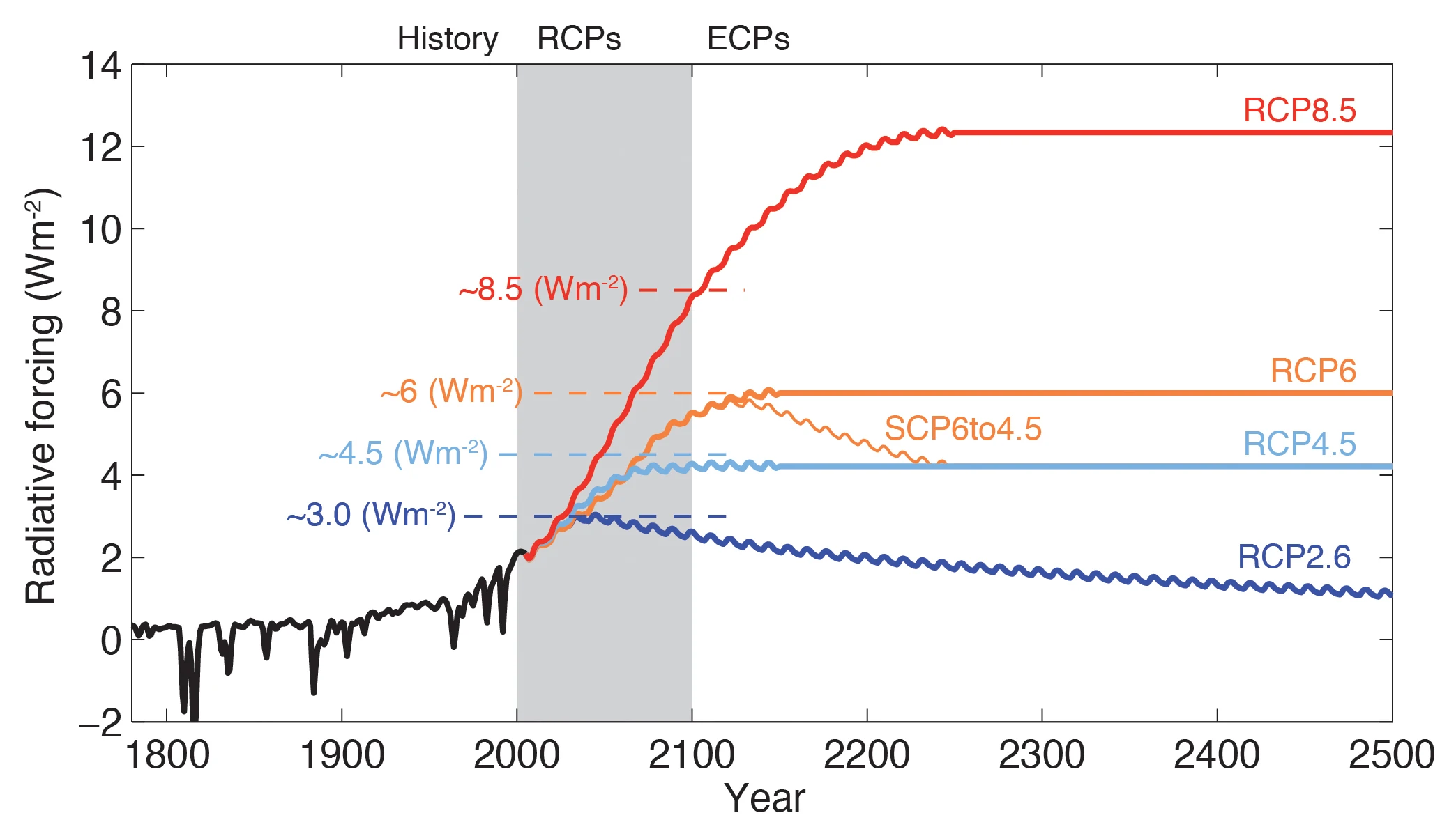
Box 1.1, Figure 1 Total RF (anthropogenic plus natural) for RCPs and extended concentration pathways (ECP)—for RCP2.6, RCP4.5, and RCP6, RCP8.5, as well as a supplementary extension RCP6 to 4.5 with an adjustment of emissions after 2100 to reach RCP4.5 concentration levels in 2250 and thereafter. Note that the stated RF levels refer to the illustrative default median estimates only. There is substantial uncertainty in current and future RF levels for any given scenario. Short-term variations in RF are due to both volcanic forcings in the past (1800–2000) and cyclical solar forcing assuming a constant 11-year solar cycle (following the CMIP5 recommendation), except at times of stabilization. (Reproduced from Figure 4 in Meinshausen et al., 2011.)
Representative Concentration Pathway (RCP) scenarios (see Section 12.3 for a detailed description of the scenarios; Moss et al., 2008; Moss et al., 2010; van Vuuren et al., 2011b) are new scenarios that specify concentrations and corresponding emissions, but are not directly based on socio-economic storylines like the SRES scenarios. The RCP scenarios are based on a different approach and include more consistent short-lived gases and land use changes. They are not necessarily more capable of representing future developments than the SRES scenarios. Four RCP scenarios were selected from the published literature (Fujino et al., 2006; Smith and Wigley, 2006; Riahi et al., 2007; van Vuuren et al., 2007; Hijioka et al., 2008; Wise et al., 2009) and updated for use within CMIP5 (Masui et al., 2011; Riahi et al., 2011; Thomson et al., 2011; van Vuuren et al., 2011a). The four scenarios are identified by the 21st century peak or stabilization value of the RF derived by the reference model (in W/m2) (Box 1.1, Figure 1): the lowest RCP, RCP2.6 (also referred to as RCP3-PD) which peaks at 3 W/m2 and then declines to approximately 2.6 W/m2 by 2100; the medium-low RCP4.5 and the medium high RCP6 aiming for stabilization at 4.5 and 6 W/m2, respectively around 2100; and the highest one, RCP8.5, which implies a RF of 8.5 W/m2 by 2100, but implies rising RF beyond that date (Moss et al., 2010). In addition there is a supplementary extension SCP6to4.5 with an adjustment of emissions after 2100 to reach RCP 4.5 concentration levels in 2250 and thereafter. The RCPs span the full range of RF associated with emission scenarios published in the peer-reviewed literature at the time of the development of the RCPs, and the two middle scenarios where chosen to be roughly equally spaced between the two extremes (2.6 and 8.5 W/m2). These forcing values should be understood as comparative labels representative of the forcing associated with each scenario, which will vary somewhat from model to model. This is because concentrations or emissions (rather than the RF) are prescribed in the CMIP5 climate model runs.
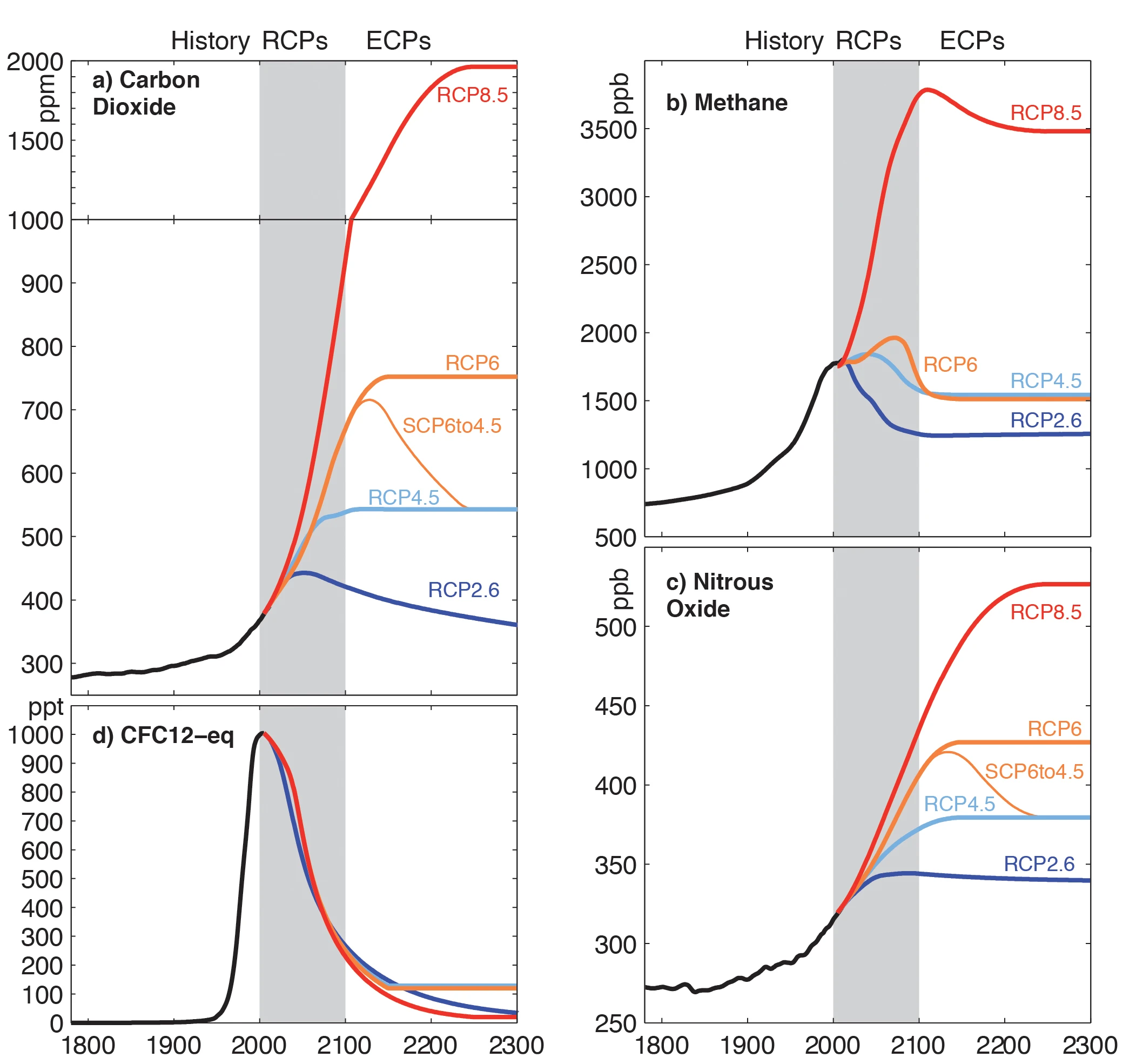
Box 1.1, Figure 2 Concentrations of GHG following the 4 RCPs and their extensions (ECP) to 2300. (Reproduced from Figure 5 in Meinshausen et al., 2011.) Also see Annex II Table AII.4.1 for CO2, Table AII.4.2 for CH4, Table AII.4.3 for N2O.
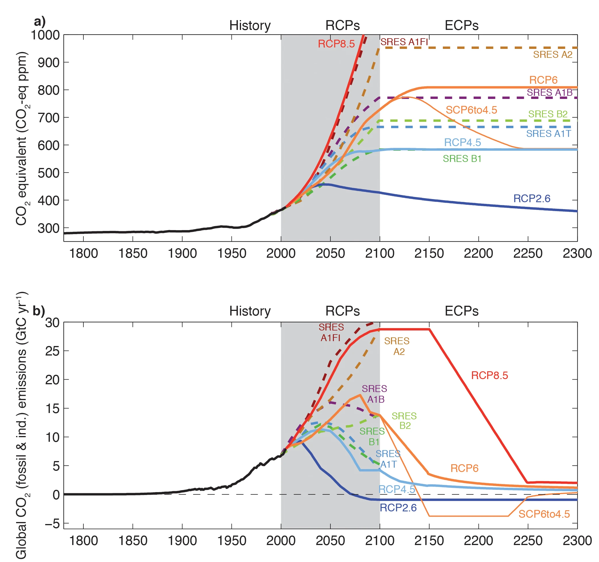
Box 1.1, Figure 3 (a) Equivalent CO₂ concentration and (b) CO₂ emissions (except land use emissions) for the four RCPs and their ECPs as well as some SRES scenarios.
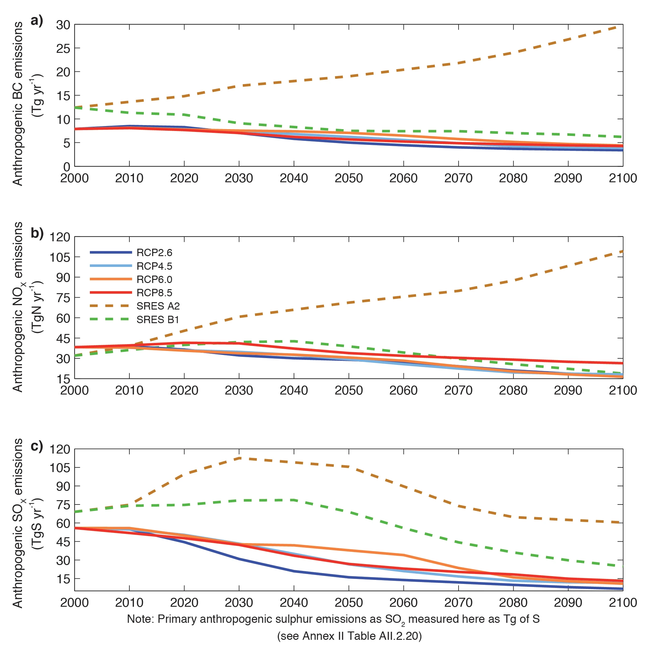
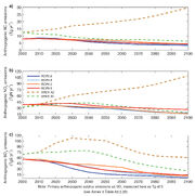
Box 1.1, Figure 4 (a) Anthropogenic BC emissions (Annex II Table AII.2.22), (b) anthropogenic NOx emissions (Annex II Table AII.2.18), and (c) anthropogenic SOx emissions (Annex II Table II.2.20).
Various steps were necessary to turn the selected ‘raw’ RCPs into emission scenarios from IAMs and to turn these into data sets usable by the climate modelling community, including the extension with historical emissions (Granier et al., 2011; Meinshausen et al., 2011), the harmonization (smoothly connected historical reconstruction) and gridding of land use data sets (Hurtt et al., 2011), the provision of atmospheric chemistry modelling studies, particularly for tropospheric ozone (Lamarque et al., 2011), analyses of 2000–2005 GHG emission levels, and extension of GHG concentrations with historical GHG concentrations and harmonization with analyses of 2000–2005 GHG concentrations levels (Meinshausen et al., 2011). The final RCP data sets comprise land use data, harmonized GHG emissions and concentrations, gridded reactive gas and aerosol emissions, as well as ozone and aerosol abundance fields (Figures 2, 3, and 4 in Box 1.1).
To aid model understanding of longer-term climate change implications, these RCPs were extended until 2300 (Meinshausen et al., 2011) under reasonably simple and somewhat arbitrary assumptions regarding post-2100 GHG emissions and concentrations. In order to continue to investigate a broad range of possible climate futures, the two outer RCPs, RCP2.6 and RCP8.5 assume constant emissions after 2100, while the two middle RCPs aim for a smooth stabilization of concentrations by 2150. RCP8.5 stabilizes concentrations only by 2250, with CO₂ concentrations of approximately 2000 ppm, nearly seven times the pre-industrial levels. As the RCP2.6 implies netnegative CO₂ emissions after around 2070 and throughout the extension, CO₂ concentrations are slowly reduced towards 360 ppm by 2300.
Comparison of SRES and RCP Scenarios[]
The four RCP scenarios used in CMIP5 lead to RF values that span a range larger than that of the three SRES scenarios used in CMIP3 (Figure 12.3). RCP4.5 is close to SRES B1, RCP6 is close to SRES A1B (more after 2100 than during the 21st century) and RCP8.5 is somewhat higher than A2 in 2100 and close to the SRES A1FI scenario (Figure 3 in Box 1.1). RCP2.6 is lower than any of the SRES scenarios (see also Figure 1.15).
ES 1.1 1.2.1 1.2.2 1.2.3 1.3 1.3.1 1.3.2 1.3.3 1.3.4 1.3.4.1 1.3.4.2 1.3.4.3 1.4.1 1.4.2 1.4.3 1.4.4 1.5 1.5.1 1.5.2 1.6 Box 1 FAQ Refs